
# Let's get the administrative stuff done first
# import all the libraries and set up the plotting

import pandas as pd
import numpy as np
from datetime import datetime,timedelta

import statsmodels.api as sm

from sklearn.cluster import KMeans, k_means
from sklearn.ensemble import BaggingClassifier, RandomForestClassifier, ExtraTreesClassifier, AdaBoostClassifier, GradientBoostingClassifier
from sklearn.ensemble import BaggingRegressor, RandomForestRegressor, ExtraTreesRegressor, AdaBoostRegressor, GradientBoostingRegressor
from sklearn.gaussian_process import GaussianProcessRegressor
from sklearn.linear_model import LogisticRegression, LogisticRegressionCV
from sklearn.linear_model import Ridge, Lasso, ElasticNet, LinearRegression, RidgeCV, LassoCV, ElasticNetCV
from sklearn.metrics import accuracy_score, mean_squared_error, silhouette_score, roc_auc_score

from sklearn.model_selection import train_test_split, cross_val_score, GridSearchCV, RandomizedSearchCV
from sklearn.neighbors import KNeighborsRegressor, KNeighborsClassifier
from sklearn.pipeline import Pipeline
from sklearn.preprocessing import StandardScaler, PolynomialFeatures
from sklearn.svm import SVC, SVR
from sklearn.tree import DecisionTreeClassifier, DecisionTreeRegressor


import matplotlib
import matplotlib.pyplot as plt
import seaborn as sns
plt.style.use('seaborn')
sns.set(style="white", color_codes=True)
colors_palette = sns.color_palette("GnBu_d")
sns.set_palette(colors_palette)

# GnBu_d
colors = ['#37535e', '#3b748a', '#4095b5', '#52aec9', '#72bfc4', '#93d0bf']
Data checking functions
# Check which non-numeric columns are missing values and what the possible values are for each object column

def check_cols(df):
    cols = df.select_dtypes([np.object]).columns
    for col in cols:
        print("{} is {} and values are {}.".format(col,df[col].dtype,df[col].unique()))
        n_nan = df[col].isnull().sum()
        if n_nan > 0:
            print("{} has {} NaNs.".format(col,n_nan))

    cols = df.select_dtypes([np.int64,np.float64,np.uint64]).columns
    for col in cols:
        print("{} is {} and values are {} to {}.".format(col,df[col].dtype,df[col].min(),df[col].max()))
        n_nan = df[col].isnull().sum()
        if n_nan > 0:
            print("{} has {} NaNs.".format(col,n_nan))
    return
# Check which numeric columns are missing values

def check_data(df):
    s = df.shape
    print("Rows: {} Cols: {}".format(s[0],s[1]))

    # Check for null values
    null_data = df.isnull().sum()
    null_data_count = sum(df.isnull().sum())
    if  null_data_count > 0:
        print("There are {} null data.".format(null_data_count))
        print("Columns with NaN: {}".format(list(null_data[null_data > 0].index)))

    duplicates = df[df.duplicated()].shape[0]
    print("There are {} duplicate rows in the test data.".format(duplicates))

    check_cols(df)

    return
def read_examine_df(file):
    df = pd.read_csv(file)
    check_data(df)
    return df
I. Define the problem
Predict when and where different species of mosquitos will test positive for West Nile virus. A more accurate method of predicting outbreaks of West Nile virus in mosquitos will help the City of Chicago and CPHD more efficiently and effectively allocate resources towards preventing transmission of this potentially deadly virus.
For each record in the test set, you should predict a real-valued probability that WNV is present.
II. Obtain the data.
- Training data: train.csv
- Test data: test.csv
- Spray data: spray.csv
- Weather data: weather.csv
Training data
- Rows: 10506
- Cols: 12
- There is NO null data.
do_check_data = False
if do_check_data:
    df_train = read_examine_df("../data/train.csv")
else:
    df_train = pd.read_csv("../data/train.csv")
Cleaning the training data
- Latitude and longitude have reasonable ranges.
- Drop all other address data for now.
- Replace Date with a datetime object.
- Create Week and Year features.
- (Removed) Merge rows with same trap/date/species; sum NumMosquitos and set WnvPresent to 0 or 1 acordingly. This may cause us to lose some information. Scott and Al convinced Gwyneth that this is a bad idea overall. There might be some value in the aggregatingg if done at the right times.
# For now, drop all the address columns since lat/lon should be enough
df_train.drop(['Address','Block','Street','AddressNumberAndStreet','AddressAccuracy'], axis=1,inplace=True)
# Make Date into datetime
df_train['Date'] = pd.to_datetime(df_train['Date'])

# Add week and Year columns
df_train['Week'] = (df_train['Date'].dt.strftime('%W')).astype(int)
df_train['Year'] = (df_train['Date'].dt.strftime('%Y')).astype(int)
(Removed) Aggregate split rows
# The model works better without aggregating, but there maybe a use for it

# Merge duplicate rows by summing NumMosquiots and WMvPresent
# df_train = df_train.groupby(['Date','Week','Year','Species','Trap','Latitude', 'Longitude'], as_index=False).sum().reindex()
# Change WnvPresent to be  0/1
# df_train['WnvPresent'] = (df_train['WnvPresent'] > 0).astype(int)
Plot mosquito totals by week and species
# This is the TOTAL mosquitos in a given week summed over all years.
df_temp = df_train.groupby(['Week','Species'], as_index=False).sum().reindex()

fg = sns.lmplot(data=df_temp, x = 'Week', y='NumMosquitos', hue='Species', fit_reg=False);
fg.fig.set_figheight(6)
fg.fig.set_figwidth(15)
fg.fig.suptitle("Total for each species per week over all years");

# Speies with West Nile Virus
species_wnv = set((df_train[df_train['WnvPresent'] > 0])['Species'])
Create "target" variables
There are TWO targets in this problem:
- First, we have to predict HOW MANY mosquitoes of each species will be in a trap on a given date.
- Then we have to predict the probablity that there will be West Nile virus present based on those counts.
# Create our targets then drop those columns

y_count_label = 'NumMosquitos'
y_count = df_train[y_count_label]

y_wnv_label = 'WnvPresent'
y_wnv = df_train[y_wnv_label]

df_train.drop(columns=[y_wnv_label,y_count_label], inplace=True)
Kaggle data
- Rows: 116293
- Cols: 11
- There is NO null data.
The instructions say that we are predicting all combinations of possible traps/dates/species, but we will only be scored on the records that match with actual tests/samples.
if do_check_data:
    df_kaggle = read_examine_df("../data/test.csv")
else:
    df_kaggle = pd.read_csv("../data/test.csv")
Cleaning the Kaggle data
- Latitude and longitude have reasonable ranges.
- Drop all other address data for now.
- Replace Date with a datetime object.
- Create Week and Year features.
- There are duplicate rows. Can we assume anything about these? We merged rows like this in training, but we need to make predictions here.
- Does not have NumMosquitos nor WnvPresent. These are what we need to predict.
- Does have Id column - later on, make this the index?
# For now, drop all the address columns since lat/lon should be enough
df_kaggle.drop(['Address','Block','Street','AddressNumberAndStreet','AddressAccuracy'], axis=1,inplace=True)

# Make Date into datetime
df_kaggle['Date'] = pd.to_datetime(df_kaggle['Date'])

# Add week and 'Year' feature
df_kaggle['Week'] = (df_kaggle['Date'].dt.strftime('%W')).astype(int)
df_kaggle['Year'] = (df_kaggle['Date'].dt.strftime('%Y')).astype(int)
# If there is a duplicate row, maybe that means we know there are more than 50 in trap?
kaggle_cols = list(df_kaggle.columns)
kaggle_cols.remove('Id')
duplicates = df_kaggle[df_kaggle.duplicated(kaggle_cols)].shape[0]
print("There are {} duplicate rows in the test data.".format(duplicates))

# There are 1533 duplicate rows in the test data.
df_kaggle.head()
Cleaning the trap data
While working to feature engineer the spraying data, we noticed that there are two traps that each have two different locations listed in the observation data. We rename these traps and also rename them in the Kaggle test data.
# Break apart duplicate traps !
df_traps_train = df_train[['Trap', 'Latitude','Longitude']].copy()
df_traps_train.drop_duplicates(inplace=True)
df_traps_train.reset_index(inplace=True)
print("There are {} traps in the test data.".format(df_traps_train.shape[0]))

# Here are the traps with duplicates
df_trap_duplicate = df_traps_train.loc[df_traps_train.duplicated('Trap')][['Trap','Latitude','Longitude']].copy()
if df_trap_duplicate.shape[0] > 0:
    print("There are {} bad traps in the training data. Now cleaning.".format(df_trap_duplicate.shape[0]))

# For each one, update the Train and Kaggle data too...
for i in df_trap_duplicate.index:
    trap = df_trap_duplicate.loc[i, "Trap"]
    lat = df_trap_duplicate.loc[i, "Latitude"]
    long = df_trap_duplicate.loc[i, "Longitude"]
    new_trap = trap + "GAS"
    df_train.loc[(df_train['Trap'] == trap)
                 & (df_train['Latitude'] == lat)
                 & (df_train['Longitude'] == long),'Trap'] = new_trap
    df_kaggle.loc[(df_kaggle['Trap'] == trap)
                 & (df_kaggle['Latitude'] == lat)
                 & (df_kaggle['Longitude'] == long),'Trap'] = new_trap

# Repeat with Kaggle data
df_traps_kaggle = df_kaggle[['Trap', 'Latitude','Longitude']].copy()
df_traps_kaggle.drop_duplicates(inplace=True)
df_traps_kaggle.reset_index(inplace=True)
print("There are {} traps in the Kaggle data.".format(df_traps_kaggle.shape[0]))

# Any more with duplicates
df_trap_duplicate = df_traps_kaggle.loc[df_traps_kaggle.duplicated('Trap')][['Trap','Latitude','Longitude']].copy()
if df_trap_duplicate.shape[0] > 0:
    print("There are {} bad traps in the Kaggle test data. Error: More cleaning needed.".format(df_trap_duplicate.shape[0]))
Spray data
- Rows: 14835
- Cols: 4
- There are 584 null data.
- There are 541 duplicate rows.
- Columns with NaN: Time
if do_check_data:
    df_spray = read_examine_df("../data/spray.csv")
else:
    df_spray = pd.read_csv("../data/spray.csv")
df_spray.head()
Missing spray time data for 2011-09-07
- Many Time values are missing but can likely be imputed.
- Spraying generally happens every 10 seconds.
- As the previous rows were the duplicate data, I'm going to guess that we should connect with 7:44:32.
- Based the spray time on the endpoints.
- Probably good enough to have the time within a small window of time.
# This spray time imputation is overkill, but it was fun to tackle.

# Get time of duplicate row
# Make it the start for the next set of columns
# fill the NaNs, *subtracting* ten seconds based on the map of the missing data

# Get time of duplicate row
series = df_spray[df_spray.duplicated() == True].index
idx = series[-1]

# Check the next row starts the Nans
# print("If it is not a NaN, we have a problem... {}".format(df_spray.loc[idx+1]['Time']))

# Assume the NaNs are in a row
null_data_count = sum(df_spray.isnull().sum())
# print("If it is not a NaN, we have a problem... {}".format(df_spray.iloc[idx+null_data_count]['Time']))
# print("If it IS a NaN, we have a problem... {}".format(df_spray.iloc[idx+null_data_count+1]['Time']))

# Make it the start for the next row
start_time = pd.to_datetime(df_spray.iloc[idx]['Time'])
times = [(start_time + timedelta(seconds=-10*i)).time().strftime('%H:%M:%S')
         for i in range(null_data_count)]

# Replace the missing times
df_spray.loc[df_spray['Time'].isnull(), 'Time'] = times

# Check that there are no longer any nulls
null_data_count = sum(df_spray.isnull().sum())
if  null_data_count > 0:
    print("There are {} null data.".format(null_data_count))
# Drop duplicate rows
df_spray.drop_duplicates(keep='last', inplace=True)
Other spray cleaning
# Turn the Date/Time into a datetime object
df_spray['DateTime'] = pd.to_datetime(df_spray['Date'] + " " + df_spray['Time'])

# Make Date into datetime
df_spray['Date'] = pd.to_datetime(df_spray['Date'])

# df_spray.drop(['Date','Time'], axis=1, inplace=True)
df_spray.head()
Weather data
- Rows: 2944
- Cols: 22
- There is NO null data.
if do_check_data:
    df_weather = read_examine_df("../data/weather.csv")
else:
    df_weather = pd.read_csv("../data/weather.csv")
Cleaning the weather data
- For now, keep only a subset of the columns: Date, WetBulb, Sunrise, Sunset, PrecipTotal.
- For the places where WetBulb is 'M', use the value from the other station.
- Get rid of Station 2, then drop Station column since all are Station 1.
- Replace Trace with 0.1.
- Change type of WetBulb and PrecipTotal.
- Change Sunrise and Sunset to a datetime object - clean the 1860(?!?) sunset.
- Change Date to datetime and add Week and Year.
# Keep only these columns
cols_keep = ['Station', 'Date', 'WetBulb', 'Sunrise', 'Sunset', 'PrecipTotal']
df_weather = df_weather[cols_keep].copy()

# Clean the data
# Replace 'M' with other station's WetBulb
# This should have error checking?
missing = df_weather[df_weather['WetBulb'] == 'M'].index
for i in missing:
    df_weather.loc[i,'WetBulb'] = df_weather.loc[i+1,'WetBulb']
if len(df_weather[df_weather['WetBulb'] == 'M'].index) > 0:
    print("More Wetbulb cleaning to do!!!")

# Get rid of Station 2, then drop Station column since all rows are Station 1
df_weather = df_weather[df_weather['Station'] == 1].copy()
df_weather.reset_index(inplace=True)
df_weather.drop(columns='Station', inplace=True)

# Replace "Trace" with 0.1
df_weather['PrecipTotal'].replace(to_replace='  T',value = '0.1', inplace=True)

# Change type
df_weather['WetBulb'] = df_weather['WetBulb'].astype(int)
df_weather['PrecipTotal'] = df_weather['PrecipTotal'].astype(float)

# Really? Rounding error?
# Should do more generalized cleaning/checking for these
df_weather['Sunset'].replace(to_replace='1860',value = '1900', inplace=True)
df_weather['Sunset'].replace(to_replace='1760',value = '1900', inplace=True)
df_weather['Sunset'].replace(to_replace='1660',value = '1900', inplace=True)

# Change Sunrise and Sunset to a datetime object
sunrise = df_weather['Date'] + " " + df_weather["Sunrise"]
df_weather['Sunrise'] = pd.to_datetime(sunrise, format="%Y-%m-%d %H%M")
sunset = df_weather['Date'] + " " + df_weather["Sunset"]
df_weather['Sunset'] = pd.to_datetime(sunset, format="%Y-%m-%d %H%M")

# Change Date to datetime and add Week and Year
df_weather['Date'] = pd.to_datetime(df_weather['Date'])
df_weather['Week'] = (df_weather['Date'].dt.strftime('%W')).astype(int)
df_weather['Year'] = (df_weather['Date'].dt.strftime('%Y')).astype(int)

df_weather.head()
Weekly data showing Number of Mosquitoes Collected in Traps vs Average Daily Rainfall
Refer to the "Average precipitation calculations" section for the code to generate this chart.
Summary of the data
For this project on mosquitos and the spread of West Nile Virus in Chicago, we were provided with three spreadsheets of data: the observations from mosquito traps around the city, weather data, and mosquito spraying data. We were also provided with a set of trap, date, and species tuples for which we were to predict the probability of finding West Nile virus.
Initial data cleaning
Training data
The training data has approximately 10K rows and 12 columns. There is no null data. The rows represent the trap observations, broken down by Trap, Date, and Species. Seven of the twelve columns refer to the location of the trap. A quick check of the ranges of the latitude and longitude of the the traps as well as a quick map of the locations confirm the accuracy of the latitude and longitude, so we dropped all other information regarding the address. The final two columns relate to the mosquitos in the trap: how many of each species were counted and a Boolean for whether or not West Nile was observed in the count.
In addition, we transformed the Date data into a datetime object in order to more easily calculate difference in days between observations and other such metrics. We also added in a column for Week and Year in order to aggregate observations.
In pursuing some feature engineering, we noticed that there were two traps (T009 and T035) that were placed in two different locations at different times. We "split" these traps and made the same change to the prediction data.
It is interesting to note that if a trap had more than 50 mosquitos in it, the observation is split into two observations. We debated whether or not to aggregate the rows. On one had, aggregating would give a better value for predicting the number of mosquitos that might be found in a trap. On the other hand, we would lose information about the number of cases of West Nile found.
Prediction data
The prediction data has approximately 116K rows (10x as many as the observations) and 11 columns. There is no null data. The rows represent the trap observations we need to predict, broken down by Id, Trap, Date, and Species; the Id is for Kaggle reporting purposes only. Seven of the eleven columns refer to the location of the trap, and, as with the training data, we drop all these except for latitude and longitude.
As with the training data, we transform the Date data into a datetime object in order to more easily calculate difference in days between observations and other such metrics. We also add in a column for Week and Year.
Also, like with the training data, there are duplicate rows (1533). Later on, as we model, we make some assumptions about what these represent.
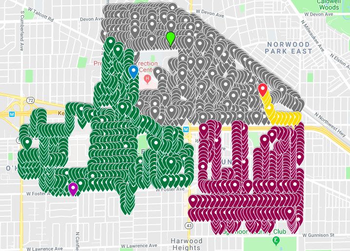
Spraying data
The spraying data has approximately 15K rows and 4 columns. The columns are Date, Time, Latitude, and Longitude. There are 450 duplicate rows and also around 450 rows that are missing Time entries. (Something went wrong in recording data.) We mapped all the spraying data, broken down by day, and all the locations appeared to be reasonable, except for the "Oops" moment on 2011-09-07.
To fix the bad spraying data, we mapped the spraying for that day, located where the observations with missing times were, and imputed the times based on noting that spraying location/time is recorded about every ten seconds. We worked harder on this than was probably necessary since spraying all happens within a small time-window.
Weather data
The weather data has approximately 3K rows and 22 columns with no missing data. The readings are taken once a day at two different stations. These observations include precipitation totals, temperature measures, sunrise, sunset, wind and humidity measurements.
For now, we only keep the columns Date, Sunrise, Sunset, WetBulb, and PrecipTotal. We also only keep the rows from the first weather station. The precipitation column has a 'T' for some entries; we changed this 'trace' into 0.1. For the 'M' readings in WetBulb, we used the data from the other station on the same day. In translating the Sunrise and Sunset times to a datetime object, we encountered that some of the times were given as 1860, etc, and needed to be corrected.
Preliminary Exploratory Data Analysis
Observation data
The dates of the observation data are approximately weekly from the end of May to the beginning of October for the years 2007, 2009, 2011, 2013. There are seven different species of mosquito in the observations, and an additional one in the set we are asked to predict. For the observations, the only Species that had West Nile Virus present were : CULEX PIPIENS', 'CULEX PIPIENS/RESTUANS', and 'CULEX RESTUANS', and there were a total of 135039 mosquitos observed. West Nile was observed 551 times.
Prediction data
The dates of the prediction data are approximately weekly from the end of May to the beginning of October for the years 2008, 2010, 2012, 2014. There are eight Species of mosquitos that we need to predict for.
Spray data
We have spraying data for ten different dates in 2011 and 2013. Spraying occurred in the evenings between 7pm and 9pm. We mapped the spray areas, and the spraying covered ten different neighborhoods.
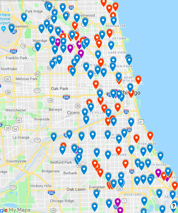
Traps data
Combining the trap data found in the observations and the prediction data, there are 151 traps (after splitting the two traps that reported two locations), spread throughout the city.
Weather data
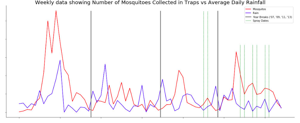
We did not have time to deeply explore the weather data. Through plotting, we visually noticed a correlation between precipitation and a spike in trap populations 3-4 weeks later.
Exploratory data analysis (EDA)
- How do we model traps NOT in training data? (Cluster?)
- We need to engineer features based on spray and weather to add to the observation data and the Kaggle test data.
- How many "categorical" features remain?
- Make dummies for all categorical data.
- Which features should we drop?
- Are there any interesting linear relationships?
New features
- Let's add a column of "Days since emptied" to indicate how long it has been since the trap was emptied.
- Let's add a column of "Days since sprayed" to indicate how long it has been since the area near the trap was sprayed.
- Since there are traps in the Kaggle test set but not in the observations set, we need to make some inferences. We chose to start by clustering the traps.
Spray data
- How long has it been since we have sprayed?
- Add a column to train/kaggle data for "Days since sprayed"?
- Are there any mosquitos in traps "near" where we spray those dates?
Create a dataframe for traps.
# What are all the traps?
df_traps_train = df_train[['Trap', 'Latitude','Longitude']].copy()
df_traps_train.drop_duplicates(inplace=True)

df_traps_kaggle = df_kaggle[['Trap', 'Latitude','Longitude']].copy()
df_traps_kaggle.drop_duplicates(inplace=True)

# Merge the dataframes and set the index to be the traps
df_traps = pd.concat([df_traps_train,df_traps_kaggle])
df_traps.drop_duplicates(inplace=True)
df_traps.set_index(['Trap'], inplace=True)

print("There are {} traps.".format(df_traps.shape[0]))
Determine dates that area near each trap was sprayed.
epsilon = .01

# Create a set of spray dates for each trap based on lat/log with epsilon
traps = list(set(df_traps.index))
traps.sort()

spray_dates = []
for t in traps:
    # This area near trap could be sprayed from this "radius"
    # Needs much improvement
    min_lat = df_traps.loc[t,'Latitude'] - epsilon
    max_lat = df_traps.loc[t,'Latitude'] + epsilon
    min_lon = df_traps.loc[t,'Longitude'] - epsilon
    max_lon = df_traps.loc[t,'Longitude'] + epsilon

    df_temp = df_spray[df_spray['Latitude'] < max_lat]
    df_temp = df_temp[df_temp['Latitude'] > min_lat]
    df_temp = df_temp[df_temp['Longitude'] < max_lon]
    df_temp = df_temp[df_temp['Longitude'] > min_lon]

    spray_dates.append(set(df_temp['Date']))

df_traps['SprayDates'] = spray_dates
Add a column to training and Kaggle dataframes for "SprayDates".
do_since_sprayed = False
if do_since_sprayed:
    df_train["SinceSprayed"] = 999

    for i in range(df_train.shape[0]):
        trap = df_train.loc[i,"Trap"]
        date = df_train.loc[i,"Date"]
        spray_dates = [d for d in df_traps.loc[trap,"SprayDates"] if d < date]
        if spray_dates:
            elapsed = (date - max(spray_dates)).days
            df_train.loc[i,"SinceSprayed"] = elapsed

    df_kaggle["SinceSprayed"] = 999

    for i in range(df_kaggle.shape[0]):
        trap = df_kaggle.loc[i,"Trap"]
        date = df_kaggle.loc[i,"Date"]
        spray_dates = [d for d in df_traps.loc[trap,"SprayDates"] if d < date]
        if spray_dates:
            elapsed = (date - max(spray_dates)).days
            df_kaggle.loc[i,"SinceSprayed"] = elapsed

    print("Minimum days since trap in training set sprayed: {}.".format(min(df_train['SinceSprayed'])))
    print("Minimum days since trap in Kaggle set sprayed: {}.".format(min(df_kaggle['SinceSprayed'])))

    # I may just use a flag to not create this column, but for now, I will drop it from training and Kaggle.
    df_train.drop(columns=['SinceSprayed'], inplace=True)
    df_kaggle.drop(columns=['SinceSprayed'], inplace=True)
*This needs some cleanup if there is time.* We spray on ten days. For each one,what are the areas that we spray that date? Which traps are near there?
- 2011-08-29 : Nothing good
- 2011-09-07 : 1 set
- 2013-07-17 : 3 sets, 2 good
- 2013-07-25 : 1 set
- 2013-08-08 : 1 set
- 2013-08-15 : 2 sets
- 2013-08-16 : 2 sets, 1 good
- 2013-08-22 : 2 sets
- 2013-08-29 : 2 sets
- 2013-09-05 : 2 sets
# Which days do we spray?
spray_dates = list(set(df_spray['Date']))
spray_dates.sort()

epsilon = .01
spray = dict()
for d in spray_dates:
    df_temp = df_spray[df_spray['Date'] == d]
    print("There are {} traps sprayed on {}.".format(df_temp.shape[0], d))

    # For dates that have dispersed spraying, this is a terrible metric!
    df_loc = df_spray[df_spray['Date'] == d]
    min_lat = min(df_loc['Latitude'])
    max_lat = max(df_loc['Latitude'])
    min_lon = min(df_loc['Longitude'])
    max_lon = max(df_loc['Longitude'])

    df_temp = df_traps[df_traps['Latitude'] < max_lat + epsilon]
    df_temp = df_temp[df_temp['Latitude'] > min_lat - epsilon]
    df_temp = df_temp[df_temp['Longitude'] < max_lon + epsilon]
    df_temp = df_temp[df_temp['Longitude'] > min_lon - epsilon]

    traps = list(set(df_temp.index))
    if len(traps) > 0:
        spray[d] = traps
Determine dates that each trap was emptied (aka observed).
# Add days since emptied to each observation/Kaggle prediction

# Gather the dates each trap was observed
obsv_dates = []
for t in df_traps.index:
    dates_train = set(df_train.loc[df_train["Trap"] == t,"Date"])
    dates_kaggle = set(df_kaggle.loc[df_kaggle["Trap"] == t,"Date"])
    obsv_dates.append(dates_train.union(dates_kaggle))
df_traps["ObsvDates"] = obsv_dates
Determine # days since trap was emptied for each observation
df_train["SinceEmptied"] = 30
for i in range(df_train.shape[0]):
    trap = df_train.loc[i,"Trap"]
    date = df_train.loc[i,"Date"]
    obsv_dates = [d for d in df_traps.loc[trap,"ObsvDates"] if d < date]
    if obsv_dates:
        elapsed = max(30,(date - max(obsv_dates)).days)
        df_train.loc[i,"SinceEmptied"] = elapsed

df_kaggle["SinceEmptied"] = 100
for i in range(df_kaggle.shape[0]):
    trap = df_kaggle.loc[i,"Trap"]
    date = df_kaggle.loc[i,"Date"]
    obsv_dates = [d for d in df_traps.loc[trap,"ObsvDates"] if d < date]
    if obsv_dates:
        elapsed = max(30,(date - max(obsv_dates)).days)
        df_kaggle.loc[i,"SinceEmptied"] = elapsed
# Drop columns to create a DataFrame from the full training set
df_train_small = df_train.copy()
df_train_small[y_count_label] = y_count
df_train_small[y_wnv_label] = y_wnv
df_train_small.drop(columns=['Latitude','Longitude','Week'], inplace=True)


for date,traps in spray.items():
    min_date = date - timedelta(days=100)
    max_date = date + timedelta(days=100)
    df_train_area = df_train_small[df_train_small["Trap"].isin(traps)].copy()
    df_train_area.drop(columns='Trap',inplace=True)
    df_train_area = df_train_area[df_train_area['Date'] >= min_date].copy()
    df_train_area = df_train_area[df_train_area['Date'] <= max_date].copy()
    df_train_area = df_train_area.groupby(['Date'], as_index=False).sum().reindex()
    df_train_area['WnvPresent'] = (df_train_area['WnvPresent'] > 0).astype(int)
    dates = list(df_train_area.loc[(df_train_area['WnvPresent'] > 0),"Date"])

    plt.figure()
    plt.plot(figsize=(10, 20))
    ax = plt.gca()
    ax.set_title(str(date))
    df_train_area.plot(x='Date', y='NumMosquitos', c=colors[0], marker='o', label = "Number of mosquitos", ax=ax);
    ax.axvline(x=date, c='r', label="Spray date")
    label = True
    for w in dates:
        if label:
            ax.axvline(x=w, c=colors[5], linestyle="dashed", label="WNV Present")
            label = False
        ax.axvline(x=w, c=colors[5], linestyle="dashed")
    ax.set_xlabel('')
    ax.set_ylabel('')
    ax.legend();


Days since last emptied
- Since there are traps in the test set but not in the train set, we need to make some inferences. We chose to start by clustering the traps.
- Set the maximum "Since emptied" to be 365.
- There must be a better way to slice the DataFrames....
- Doesn't seem to help right now, but keeping it in case we create something else that makes it so this helps.
# For each trap, calculate days since it was emptied
# There must be a more elegant way to do this using slicing, but I couldn't figure it out quickly.

do_days_since_empty = False
if do_days_since_empty:
    df_traps = pd.DataFrame(list(set(df_train['Trap']) | set(df_kaggle['Trap'])), columns=['Trap'])
    df_traps

    traps = list(df_traps['Trap'])
    dates = []
    for t in traps:
        dates_train = set(df_train.loc[df_train['Trap'] == t, 'Date'])
        dates_kaggle = set(df_kaggle.loc[df_kaggle['Trap'] == t, 'Date'])
        dates.append(dates_train | dates_kaggle)

    df_traps['Dates'] = dates
    df_traps.set_index(['Trap'], inplace=True)

    # Now for each train and kaggle record, add a column of last day checked
    emptied = []
    for i in range(df_train.shape[0]):
        trap = df_train.loc[i,"Trap"]
        date = df_train.loc[i,"Date"]
        dates = [i for i in set(df_traps.loc[trap]["Dates"]) if i < date]
        if len(dates) > 0:
            emptied_i = min((date - max(dates)).days,365)
        else:
            emptied_i = 365
        emptied.append(emptied_i)

    df_train["Emptied"] = emptied

    emptied = []
    for i in range(df_kaggle.shape[0]):
        trap = df_kaggle.loc[i,"Trap"]
        date = df_kaggle.loc[i,"Date"]
        dates = [i for i in set(df_traps.loc[trap]["Dates"]) if i < date]
        if len(dates) > 0:
            emptied_i = min((date - max(dates)).days,365)
        else:
            emptied_i = 365
        emptied.append(emptied_i)

    df_kaggle["Emptied"] = emptied
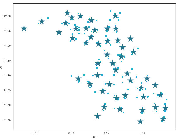
Cluster the traps
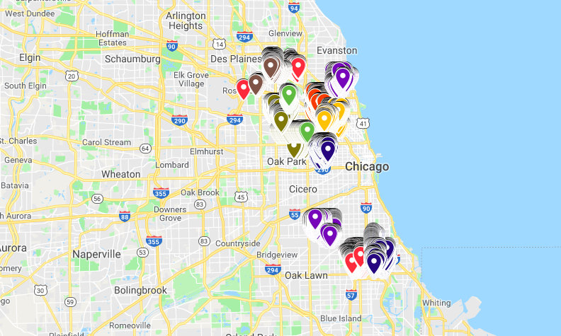
- Traps in train (orange).
- Traps in train with West Nile present (blue).
- Traps in Kaggle test (purple).
do_clusters = False

if do_clusters:
    # Combine train and test traps
    traps = df_train[['Latitude', 'Longitude']].copy()
    train_rows = traps.shape[0]
    traps = traps.append(df_kaggle[['Latitude', 'Longitude']])

    # Call k-means to cluster the traps
    kmeans = KMeans(n_clusters=50, random_state=1929)
    model = kmeans.fit(traps)
    centroids = pd.DataFrame(model.cluster_centers_, columns = ['x1', 'x2'])

    # Plot the traps and centroids

    ax = traps.plot(
        kind="scatter",
        y='Latitude', x='Longitude',
        figsize=(10,8),
        c = colors[3]
    )

    centroids.plot(
        kind="scatter",
        y="x1", x="x2",
        marker="*", s=550,
        color = colors[1],
        ax=ax
    );

    # Add the cluster information to each row
    traps['Cluster'] = kmeans.labels_
    df_train['Cluster'] = (traps['Cluster'][0:train_rows]).astype(object)
    df_kaggle['Cluster'] = (traps['Cluster'][train_rows:]).astype(object)
Create a table of Number of Mosqitos per week
Useful for plotting and mapping and feature engineering.
num_mosquito_cols = ['Year', 'Week']
df_num_mosquitos = df_train[num_mosquito_cols].copy()
df_num_mosquitos[y_count_label] = y_count
df_num_mosquitos = df_num_mosquitos.groupby(by = ['Year','Week'], as_index=False).sum()
print("Number of Weeks with mosquito counts: {}".format(df_num_mosquitos.shape[0]))
df_num_mosquitos.head()
# df_num_mosquitos.to_csv('../data/weekly_num_mosq.csv')
Function to make dummies
# Let's make dummies for the categorical data
def make_dummies(train, test, cols):

    train = train[X_cols].copy()
    test = test[X_cols].copy()

    train = pd.get_dummies(train)
    test = pd.get_dummies(test)

    # Get dummies could leave us with mismatched columns
    # Make sure we have mathcing columns in the train and kaggle DataFrames

    cols_train = train.columns
    cols_test = test.columns

    for c in cols_train:
        if c not in cols_test:
            test[c] = 0

    for c in cols_test:
        if c not in cols_train:
            train[c] = 0

    columns = sorted(train.columns)
    train = train[columns]
    test = test[columns]

    if train.shape[1] != test.shape[1]:
        print("Train and Test don't have same # columns: {} {}".format(train.shape[1], test.shape[1]))

    # Having made dummies, we now have lots and lots of columns
    print("There are {} columns and {} categorial columns."
          .format(train.shape[1],
                  train.select_dtypes([np.object]).shape[1]))

    return [train, test]
Feature engineering
Traps
For each trap, we calculated two sets: the days it was emptied and the days it was sprayed. The first one is fairly straightforward to compute from the observations. The second took more work as we needed to create a distance metric to determine if a trap was in an area covered by spraying. From these, we were able to add columns to the observations and predictions: Days since sprayed (Since_sprayed) and Days since emptied (Since_emptied).
Clusters
Considering how account for the fact that we had to predict data for traps not in the observation set, we decided to see if we could create a category column in the observation and prediction data for "clusters" of traps. An elegant process and map, but unfortunately did not appear to give us any extra benefit in the end. The latitude and longitude measures were sufficient.
Make dummies
While much of the data is numerical, there is some categorical data (Species, in particular) that we needed to make dummy columns for. As always, we had to ensure that both the observations and predictions had the same dummies.
Model the data
For each record in the test set, you should predict a real-valued probability that WNV is present.
- First, we have to predict HOW MANY mosquitoes of each species will be in a trap on a given date.
- Then we have to predict the probablity that there will be West Nile virus present based on those counts.
We had two models:
- For both steps, we tried a Grid Search on a Pipeline.
- Computing a dataframe with empirical probalities of WNV | # in trap & species. See the section below.
The MASSIVE Pipeline
- The Pipeline function takes a set of features and a model and runs grid search over their parameters on the train/test data for the specified model.
- Adjustment of the parameter ranges is not automated at this time. Each time it runs, we check to see if a parameter bound has been hit and adjust the value ranges.
- The function returns information about the best model, but not the model itself. Perhaps to be included in the future.
def run_pipline(items, X_train, X_test, y_train, y_test):

    # Add a pipe, add a param !
    pipe_items = {
        'ss' : StandardScaler(),
        'pf' : PolynomialFeatures(),

        'lr' : LinearRegression(),
        'rd' : Ridge(),
        'la' : Lasso(),
        'en' : ElasticNet(),
        'gr' : GaussianProcessRegressor(),
        'rf' : RandomForestRegressor(),
        'gb' : GradientBoostingRegressor(),
        'ab' : AdaBoostRegressor(),
        'svm' : SVR(),
        'knn' : KNeighborsRegressor(),

        'lgr' : LogisticRegression(),
        'rfc' : RandomForestClassifier(),
        'gbc' : GradientBoostingClassifier(),
        'abc' : AdaBoostClassifier(),
        'svc' : SVC(),
        'knnc' : KNeighborsClassifier()

    }

    # Include at least one param for each pipe item
    param_items = {
        'ss' : {
            'ss__with_mean' : [False]
        },
        'pf' : {
            'pf__degree' : [2]
        },
        'lr' : {
            'lr__n_jobs' : [1]
        },
        'rd' : {
             'rd__alpha' : [55.0, 60.0, 65.0]
        },
        'la' : {
             'la__alpha' : [0.005, 0.0075, 0.01],
             'la__max_iter' : [100000]
        },
        'en' : {
             'en__alpha' : [0.01, 0.02, 0.4],
             'en__l1_ratio' : [.8, 1, 1.2]
        },
        'gr' : {
            'gr__alpha' : [1, 0.1]
        },
        'rf' : {
            'rf__n_estimators' : [7, 8, 9]
        },
        'gb' : {
            'gb__n_estimators' : [325, 330, 335]
        },
        'ab' : {
            'ab__n_estimators' : [65, 70, 75]
        },
        'svm' : {
            'svm__kernel' : ['linear','poly']
        },
        'knn' : {
            'knn__n_neighbors' : [3, 4, 5, 6]
        },
        'lgr' : {
            'lgr__C' : [.04, .05, .06],
            'lgr__penalty' : ['l1','l2']
        },
        'rfc' : {
            'rfc__n_estimators' : [7, 8, 9, 10]
        },
        'gbc' : {
            'gbc__n_estimators' : [35, 40, 45]
        },
        'abc' : {
            'abc__n_estimators' : [80, 90, 100]
        },
        'svc' : {
            'svc__kernel' : ['linear','poly']
        },
        'knnc' : {
            'knnc__n_neighbors' : [35, 40, 45, 50]
        }

    }

    # Create the parameters for GridSearch
    params = dict()
    for i in items:
        for p in param_items[i]:
            params[p] = param_items[i][p]

    # Create the pipeline
    pipe_list = [(i,pipe_items[i]) for i in items]
    print("Using:")
    for p in pipe_list:
        print("\t" + str(p[1]).split('(')[0])
    pipe = Pipeline(pipe_list)

    # Grid search
    gs = GridSearchCV(pipe, param_grid=params, verbose=1)
    gs.fit(X_train, y_train)

    # Print the results
    train_params = gs.best_params_
    train_score = gs.best_score_
    y_test_hat = gs.predict(X_test)
    test_score = gs.score(X_test, y_test)

    for k in train_params:
        print("{}: {}".format(k,train_params[k]))

    print("Train score: {} Test score {}".format(train_score, test_score))
    print("")

    return train_score, test_score, y_test_hat, train_params
Prepare for REGRESSION to predict NumMosquitos
- Use a subest of columns: The columns are ['Week', 'Year', 'Species', 'Latitude', 'Longitude']
- Make dummies on the columns (only 'Species' at the moment).
- Do a train/test split on the training data.
# Let's start with a few features
X_cols = list(df_train.columns)
X_cols.remove('Date')
X_cols.remove('Trap')

if do_days_since_empty:
    X_cols.remove('Emptied')

if do_clusters:
    X_cols.remove('Latitude')
    X_cols.remove('Longitude')

print("The columns are {}".format(X_cols))
[X_cols_train, X_cols_kaggle] = make_dummies(df_train, df_kaggle, X_cols)

# Test/train split of "full training" data
X_train, X_test, y_train, y_test = train_test_split(X_cols_train, y_count, random_state=42)
Call the pipeline to use REGRESSION to predict NumMosquitos
- Choose a regression model.
- Use StandardScaler.
- Update params values based on grid search and repeat (not automated).
- Fudge the predicted data -- NumMosquitos is non-negative and if duplicate rows in Kaggle test data, all but last row should have 50 mosquitos.
# Regression models
# 'lr' : LinearRegression(),
# 'rd' : Ridge(),
# 'la' : Lasso(),
# 'en' : ElasticNet(),
# 'gr' : GaussianProcessRegressor(),
# 'rf' : RandomForestRegressor(),
# 'gb' : GradientBoostingRegressor(),
# 'ab' : AdaBoostRegressor(),
# 'svm' : SVR(),
# 'knn' : KNeighborsRegressor(),

models = ['lr','rd','la','en','rf','gb','ab','knn'] # 'gr',svm']

model_solns = {}
for m in models:
    pipe_items = ['ss', m]
    [train_score, test_score, y_test_hat, best_params] = run_pipline(pipe_items,
                                                            X_train, X_test,
                                                            y_train, y_test)
    model_solns[idx] = {'model': m,
                        'train_score': train_score, 'test_score': test_score,
                        'best_params': best_params, 'y_test_hat' : y_test_hat}
Choose best REGRESSION to predict NumMosquitos
- The best regression model is GradientBoostingRegressor.
- Using the best model, predict the NumMosquitos for the Kaggle test set.
- Do a little post-processing to the predicted counts.
Fit the best model to the training set.
pipe = Pipeline([
    ('ss', StandardScaler()),
    ('gb', GradientBoostingRegressor())
])
params_grid_cv = {
    'ss__with_mean' : [False],
    'gb__n_estimators' : [325, 330, 335]
}

gs = GridSearchCV(pipe, param_grid=params_grid_cv, verbose=1)
gs.fit(X_train, y_train)

# Predict the sales price of the Kaggle data
y_hat = gs.predict(X_test)

print("Train score: {} Test score: {}".format(gs.score(X_train,y_train),gs.score(X_test,y_test)))

# With aggregating observation rows:
# Train score: 0.9837199209535019 Test score: 0.9560608932255188

# Train score: 0.5849628964570315 Test score: 0.5677847042206758
Fit the model to the Kaggle set and add the predictions to the Kaggle test DataFrame.
# Fit full train data to predict kaggle
# Didn't help
# gs.fit(X_cols_train,y_count)

# Now predict how many mosquitoes will be in each of the kaggle tests given this
df_train[y_count_label] = y_count
df_kaggle[y_count_label] = gs.predict(X_cols_kaggle)
Duplicate rows should have 50 mosquitos.
# 50 in all duplicates except the "last" duplicate
# Replace negative values with 0

# Remove the Id
cols = list(df_kaggle.columns)
cols.remove('Id')

# Indices of duplicates for the first occurrence
duplicate_indices = df_kaggle[df_kaggle.duplicated(cols) == True].index

# There are 50 mosquitos in the "previous" record
for i in duplicate_indices:
    df_kaggle.loc[i-1,y_count_label] = 50
The number of mosquitos should be non-negative.
df_kaggle.loc[(df_kaggle[y_count_label] < 0), y_count_label] = 0
Prepare for CLASSIFICATION to predict if West Nile is present given the NumMosquitos.
- Use a subest of columns: The columns are ['Week', 'Species', 'Latitude', 'Longitude', 'Year', 'NumMosquitos']
- Make dummies on the columns (only 'Species' at the moment).
- Do a train/test split on the training data.
# Let's start with a few features
X_cols = list(df_train.columns)
X_cols.remove('Date')
X_cols.remove('Trap')
# X_cols.remove('Year')

if do_clusters:
    X_cols.remove('Latitude')
    X_cols.remove('Longitude')

print("The columns are {}".format(X_cols))
[X_cols_train, X_cols_kaggle] = make_dummies(df_train, df_kaggle, X_cols)

# Test/train split of "full training" data
X_train, X_test, y_train, y_test = train_test_split(X_cols_train, y_wnv, random_state=42)
Call the pipeline to use CLASSIFICATION to predict if West Nile is present given the NumMosquitos.
- Choose a classification model.
- Use StandardScaler.
- Update params values based on grid search and repeat (not automated).
# Classification models
#         'lgr' : LogisticRegression(),
#         'rfc' : RandomForestClassifier(),
#         'gbc' : GradientBoostingClassifier(),
#         'abc' : AdaBoostClassifier(),
#         'svc' : SVC(),
#         'knnc' : KNeighborsClassifier()

# Decide what to put into the pipline, grid searh, and save the "best" for each grid search
models = ['lgr','rfc','gbc','abc','knnc']
# other = ['pf','ss']

# After some initial tests, these seem like the best to pursue further
# models = ['lgr']

model_solns = {}
for m in models:
    pipe_items = ['ss', m]
    [train_score, test_score, y_test_hat, best_params] = run_pipline(pipe_items,
                                                            X_train, X_test,
                                                            y_train, y_test)
    model_solns[idx] = {'model': m,
                        'train_score': train_score, 'test_score': test_score,
                        'best_params': best_params, 'y_test_hat' : y_test_hat}
pipe = Pipeline([
    ('ss', StandardScaler()),
    ('lgr', LogisticRegression())
])
params_grid_cv = {
    'ss__with_mean' : [False],
    'lgr__C' : [.04, .05, .06],
    'lgr__penalty' : ['l1','l2']
}


gs = GridSearchCV(pipe, param_grid=params_grid_cv, verbose=1)
gs.fit(X_train, y_train)

# Predict the sales price of the Kaggle data
y_test_hat = gs.predict(X_test)
y_test_proba = gs.predict_proba(X_test)
df_test_proba = pd.DataFrame(y_test_proba)
y_test_proba = df_test_proba[1]

print("Train score: {} Test score: {}".format(gs.score(X_train,y_train),gs.score(X_test,y_test)))
print("ROC AUC score: {}".format(roc_auc_score(y_test, y_test_proba)))

# Train score: 0.947074501840335 Test score: 0.9489912447658927
# ROC AUC score: 0.779049996707198
Modeling
The main objective For each entry in the predictions dataset, we need to predict the probability that West Nile will be observed.
Model 1: Regression/Classification with post-processing
The initial idea for a model was to break it into two steps: first predict how many of each species would be in a trap for each entry in the predictions data set, then from that predict the probability of West Nile.
For the first model, we took a subset of the features('Week', 'Year', 'Species', 'Latitude', 'Longitude'), did a train/test split on the observed data, and then ran a grid search including scaling using eight different regression algorithms on the data in order to predict HOW MANY mosquitos of each species will be present. The best regressor was the GradientBoostingRegressor. Once a model was fit and the parameters tuned, we then made a prediction.
We then tuned this mosquito count prediction in two ways. First, we rounded up to 0 any negative predictions. Second, we made the observation that there were 1533 duplicate rows in the Kaggle test data set. ASSUMING, that this is for the same reasons there were duplicate rows in the observation set, we set the predicted number of mosquitos to be 50 for the duplicate row (except for the last duplicate in each repetition.
Given our new "feature" of "Number of Mosquitos", we then took a subset of the features('Week', 'Year', 'Species', 'Latitude', 'Longitude', 'NumMosquitos'), did a train/test split on the observed data, and then ran a grid search including scaling using six different classification algorithms on the data in order to predict the PRESENCE of West Nile Virus for each Kaggle test observation. The best classification was LogiticRegression. Once a model was fit and the parameters tuned, we then make a prediction on the probability that for the date/trap/species there will be a positive test for West Nile Virus.
We then tuned this probability prediction by setting the prediction to 0.0 for all species OTHER that the three in which West Nile was observed. (This is done below right now, but could be moved up.)
This gave an AUC ROC of 0.78. On Kaggle, the scores are 0.72432 and 0.73532. (../data/model_preds_2018-09-20 17/01/32.671403.csv)
Model 2: Percentage model
The percentage model leverages the modeling done above with respect to the prediction of the number of mosquitoes present in the Kaggle test traps. We then sought to create data from our data files so that we could look up the probability of the presence of West Nile given the species found in the that trap and the number of mosquitoes present in the trap.
There are three species of mosquitoes that carried West Nile virus in our observations. We summed the data available to create a matrix of the number of observations where the columns are the species and the rows are the number of mosquitoes found in the trap. We then created a second, similar matrix except that the observations where only the times that West Nile virus was present. The final matrix is the division of the second by the first. This gives the probability of finding West Nile virus in a trap given the number of mosquitoes in the trap of a certain species.
The results were choppy by number of mosquitoes but generally followed an upward trend. For the three species where West Nile virus was present, we then used linear regression tools to smooth the probabilities (least squares line of best fit). By linking the Kaggle test data (species plus projected mosquitoes using GradientBosstingRegression) to these smoothed probabilities, we could complete a submission file.
Using this final, smoothed result gave an AUC ROC of 0.71 (../data/sub0007.csv).
# Fit full train data to predict kaggle
# Didn't help
# gs.fit(X_cols_train,y_wnv)

y_kaggle_proba = gs.predict_proba(X_cols_kaggle)
y_kaggle = list(y_kaggle_proba[:,1])
# Create dataframe for Kaggle submission
# Make the ID the index
df_kaggle['WnvPresent'] = y_kaggle
df_kaggle.loc[(df_kaggle['Species'].isin(species_wnv) == False), 'WnvPresent'] = 0
y_kaggle = df_kaggle['WnvPresent']
df_kaggle.set_index("Id", inplace=True)
df_soln = pd.DataFrame(df_kaggle.index)
df_soln['WnvPresent'] = y_kaggle

# Predict no Wnv if not one of three species
df_soln.set_index(['Id'], inplace=True)
# Write predicted Kaggle solution out to a file
now = str(datetime.now())
f'predictions_{now}'
df_soln.to_csv(f'../data/model_preds_{now}.csv')
import matplotlib.pyplot as plt
import numpy as np
import pandas as pd
import datetime
import time

import scipy.stats as stats

from sklearn.cluster import KMeans, k_means
from sklearn.metrics import silhouette_score
from sklearn.model_selection import train_test_split
from sklearn.tree import DecisionTreeClassifier

pd.set_option('display.max_columns', 500)
pd.set_option('display.max_rows', 999)

%matplotlib inline
kaggle_train = pd.read_csv('../data/train.csv')
kaggle_test = pd.read_csv('../data/test.csv')

X_k_train = kaggle_train[['Date', 'Species', 'Trap', 'Latitude', 'Longitude', 'NumMosquitos','WnvPresent']].copy()
X_cols = list(X_k_train.columns.drop(['WnvPresent','NumMosquitos']))

X_k_train['Date'] = pd.to_datetime(kaggle_train['Date'])

X_k_train.head()
spec = list(set(X_k_train['Species']))
df = pd.DataFrame(0, index = range(51), columns = spec)
df.head()
def add_to_df(df_in, species, yn_var):
    df_in.loc[yn_var,species] += 1
    return(df_in)

for each in range(len(X_k_train)):
    df = add_to_df(df, X_k_train.loc[each,'Species'], X_k_train.loc[each,'NumMosquitos'])

df.head()       # number of occurance of species / trap in the training data
def add_to_df2(df_in, species, NumM, Wnv):
    df_in.loc[NumM,species] += Wnv
    return(df_in)

df2 = pd.DataFrame(0, index = range(51), columns = spec)
for each in range(len(X_k_train)):
    df2 = add_to_df2(df2, X_k_train.loc[each,'Species'], X_k_train.loc[each,'NumMosquitos'],X_k_train.loc[each,'WnvPresent'])

df2.head()           # number of WNV Present occurances by Species and Number in trap
df3 = df2.copy()
for i in range(len(df2)):
    for j in df2.columns:
        if df.loc[i,j] == 0:
            df3.loc[i,j] = 0
        else:
            df3.loc[i,j] = df2.loc[i,j] / df.loc[i,j]

df3.head()     # Empirical probabilities of WNV present given Species and Number of Mosquitos in trap
Creating a regression to smooth the probabilities given species & trap number
X = list(range(0,51))
y = df3['CULEX PIPIENS']
slope, intercept, r_value, p_value, std_err = stats.linregress(X,y)


probs = pd.DataFrame(0, index = range(51), columns = set(kaggle_test['Species']))
prob = []
for each in X:
    prob.append(each*slope+intercept)

    prob[0] = 0
probs['CULEX PIPIENS'] = prob

y = df3['CULEX PIPIENS/RESTUANS']
slope, intercept, r_value, p_value, std_err = stats.linregress(X,y)
prob = []
for each in X:
    prob.append(each*slope+intercept)
prob[0] = 0
probs['CULEX PIPIENS/RESTUANS'] = prob

y = df3['CULEX RESTUANS']
slope, intercept, r_value, p_value, std_err = stats.linregress(X,y)
prob = []
for each in X:
    prob.append(each*slope+intercept)
prob[0] = 0
probs['CULEX RESTUANS'] = prob

probs
Read projected mosquito by trap and species and match each projection data row with a probability
k = pd.read_csv('../data/pred_mosq.csv')

k['WnvPresent'] = 0

for each in range(len(k)):
    sp = k.loc[each, 'Species']
    num = int(k.loc[each, 'NumMosquitos'])
    k.loc[each, 'WnvPresent'] = probs.loc[num,sp]
    if sp == 'UNSPECIFIED CULEX':
        kaggle_test.loc[each, 'WnvPresent'] = .01

out = k[['Id', 'WnvPresent']]
out.to_csv('../data/sub007.csv', index = False)
Make a couple of graphs for presentation
# Change labels as needed
ax = df3['CULEX RESTUANS'].plot(kind='line', c='b', figsize = (12,8), label = 'Culex Restuans Raw')
ax = probs['CULEX RESTUANS'].plot(kind='line', c='g', figsize = (12,8), label = 'Culex Restuans Smoothed')
ax.spines['right'].set_visible(False)
ax.spines['top'].set_visible(False)
plt.legend(loc = 'upper left', fontsize = 18);
import matplotlib.pyplot as plt
import numpy as np
import pandas as pd
import datetime
import time
from sklearn.model_selection import train_test_split
from sklearn.tree import DecisionTreeClassifier

pd.set_option('display.max_columns', 500)
pd.set_option('display.max_rows', 999)

%matplotlib inline
weather = pd.read_csv('../data/weather.csv', skipinitialspace=True)

weather['Date'] = pd.to_datetime(weather['Date'])
weather[weather['PrecipTotal'] =='M']
weather.loc[117,'PrecipTotal'] = 0
weather.loc[119,'PrecipTotal'] = 0

weather['year'] = weather['Date'].dt.strftime('%Y')
weather['week'] = weather['Date'].dt.strftime('%W')
df = pd.DataFrame(pd.to_numeric(weather['year']))
df['week'] = pd.to_numeric(weather['week'])
df['precip'] = pd.to_numeric(weather['PrecipTotal'].replace('  T',0))

df_prec = (df.groupby(by = ['year','week']).mean())
(df.groupby(by = ['year','week']).mean()).to_csv('../data/weekly_precip.csv')
df_prec = df_prec.reset_index()
train_full = pd.read_csv('../data/train.csv')
train = train_full[['Date', 'NumMosquitos']].copy()
train['Date'] = pd.to_datetime(train['Date'])
train['year'] = train['Date'].dt.strftime('%Y')
train['week'] = train['Date'].dt.strftime('%W')
train['year'] = pd.to_numeric(train['year'])
train['week'] = pd.to_numeric(train['week'])

train = train.drop(['Date'], axis = 1)
(train.groupby(by = ['year','week']).sum()).to_csv('../data/weekly_num_mosq.csv')

df_numb = (train.groupby(by = ['year','week']).sum())
df_numb = df_numb.reset_index()
full_merge = pd.merge(df_prec, df_numb, how='left', on=['year','week'])
dropna_merge = full_merge.dropna().reset_index()
dropna_merge.head()

#fig = plt.figure(figsize = (12, 6))

figsize=(20, 8)
ax = dropna_merge['NumMosquitos'].plot(kind = 'line', c = 'r', figsize=figsize, label = 'Mosquitos')
ax = (dropna_merge['precip']*10000).plot(kind = 'line', c = 'b', figsize=figsize, label = 'Rain')
plt.axvline(17.5, c = 'grey', lw = 3, ymax = .95, label = "Year Breaks ('07, '09, '11, '13)")
plt.axvline(34.5, c = 'grey', lw = 3, ymax = .95)
plt.axvline(48.5, c = 'grey', lw = 3, ymax = .95)

plt.axvline(45, c = 'g', lw = 1, ls = 'dashed', ymax = .95, label = 'Spray Dates')
plt.axvline(46, c = 'g', lw = 1, ls = 'dashed', ymax = .95)
plt.axvline(54, c = 'g', lw = 1, ls = 'dashed', ymax = .65)
plt.axvline(55, c = 'g', lw = 1, ls = 'dashed', ymax = .65)
plt.axvline(57, c = 'g', lw = 1, ls = 'dashed', ymax = .65)
plt.axvline(58, c = 'g', lw = 1, ls = 'dashed', ymax = .65)
plt.axvline(60, c = 'g', lw = 1, ls = 'dashed', ymax = .65)
plt.axvline(61, c = 'g', lw = 1, ls = 'dashed', ymax = .65)


plt.title('Weekly data showing Number of Mosquitoes Collected in Traps vs Average Daily Rainfall', fontsize = 20)
ax.spines['right'].set_visible(False)
ax.spines['top'].set_visible(False)
ax.spines['right'].set_visible(False)
ax.spines['top'].set_visible(False)
ax.set_yticklabels([])
ax.set_xticklabels([])
plt.legend(loc = 'upper right');
Future investigations:
Includes but not limited to:
- Re-add dates checked column for each trap.
- Clean up the calculation of Sprayed Date - so messy.
- Re-add a column for time since last observation for each trap.
- Check if every trap was checked on each date.
- Improve distance calculation for determining if a trap was within the spraying radius
- Investigate hours of daylight.
- Explore the weather data more deeply. Dates, streaks, etc.
- Dig further into spraying data as well.
- Observations with zero of a species. Should we add an extra row just in case? Will that actaully add any new information?
- Cleanup spray graphics.
- Are there any interesting linear relationships?
- More graphs of spray and weather and mosquito information over time
- Include distribution of WNV and species over each summer.
- Tune the regression/classification algorithms and add more?
- Try to fit ExtraTrees, Gamma GLM.
- Investigate unbalanced data and how best to account for it.
- Extend the grid search to search over all combinations of regression/classifications for the two steps in the model.
- Aggregate the observations to predict the # of mosquitos in a top, then split to predict probability of West Nile. If we aggregate, we lose some info. But if we don't aggregate, we run the risk of under-predicting the number of mosquitos. I think we should try aggregating to predict counts, then unaggregating to predict the presence
# Calculating the hotspots
def put_t_back(obs_in):
    obs_in = str(obs_in)
    if len(obs_in) == 1:
        obs_out = 'T00'+obs_in
    if len(obs_in) == 2:
        obs_out = 'T0'+obs_in
    if len(obs_in) == 3:
        obs_out = 'T'+obs_in
    return(obs_out)

hotspot_traps = []
for each in traps_with_highest_WNV:
    hotspot_traps.append(put_t_back(each))
# Calculate disdance from lat/lon

from math import radians, cos, sin, asin, sqrt

def haversine(lat1, lon1, lat2, lon2):
    """
    Calculate the great circle distance between two points
    on the earth (specified in decimal degrees)
    """
    # convert decimal degrees to radians
    lon1, lat1, lon2, lat2 = map(radians, [lon1, lat1, lon2, lat2])

    # haversine formula
    dlon = lon2 - lon1
    dlat = lat2 - lat1
    a = sin(dlat/2)**2 + cos(lat1) * cos(lat2) * sin(dlon/2)**2
    c = 2 * asin(sqrt(a))
    r = 3956 # Radius of earth in kilometers = 6371. Use 3956 for miles
    return c * r
# # Only three species have West Nile
# # Export DataFrame to map
# df_wnv = df_train[df_train['WnvPresent'] == 1]
# print("Species with West Nile virus: {}.".format(set(df_wnv['Species'])))
# Linear Regression can't handle datetime
# X_cols_train['Date'] = X_cols_train['Date'].map(datetime.toordinal)
# X_cols_kaggle['Date'] = X_cols_kaggle['Date'].map(datetime.toordinal)
# # These are only used for creating the map and not part of the notebook flow

# # Used to plot traps
# df_traps = df_kaggle[['Trap','Latitude','Longitude']]
# df_traps.drop_duplicates(inplace=True)
# df_traps.shape
# df_traps.to_csv(f'../data/traps_kaggle.csv')

# # Get the traps and export to map
# df_traps = df_train[['Trap','Latitude','Longitude']]
# df_traps.drop_duplicates(inplace=True)
# df_traps.shape
# df_traps.to_csv(f'../data/traps_train.csv')
# # These are only used for creating the map and not part of the notebook flow

# # ['2011-08-29' '2011-09-07' '2013-07-17' '2013-07-25' '2013-08-08'
# #  '2013-08-15' '2013-08-16' '2013-08-22' '2013-08-29' '2013-09-05']

# df_1 = df_spray[df_spray['Date'] == '2011-08-29']
# df_1['DateTime'] = pd.to_datetime(df_1['Date'] + " " + df_1['Time'])
# df_1.to_csv(f'../data/spray-2011-08-29.csv')

# df_3 = df_spray[df_spray['Date'] == '2013-07-17']
# df_3['DateTime'] = pd.to_datetime(df_3['Date'] + " " + df_3['Time'])
# df_3.to_csv(f'../data/spray-2013-07-17.csv')

# df_4 = df_spray[df_spray['Date'] == '2013-07-25']
# df_4['DateTime'] = pd.to_datetime(df_4['Date'] + " " + df_4['Time'])
# df_4.to_csv(f'../data/spray-2013-07-25.csv')

# df_5 = df_spray[df_spray['Date'] == '2013-08-08']
# df_5['DateTime'] = pd.to_datetime(df_5['Date'] + " " + df_5['Time'])
# df_5.to_csv(f'../data/spray-2013-08-08.csv')

# df_6 = df_spray[df_spray['Date'] == '2013-08-15']
# df_6['DateTime'] = pd.to_datetime(df_6['Date'] + " " + df_6['Time'])
# df_6.to_csv(f'../data/spray-2013-08-15.csv')

# df_7 = df_spray[df_spray['Date'] == '2013-08-16']
# df_7['DateTime'] = pd.to_datetime(df_7['Date'] + " " + df_7['Time'])
# df_7.to_csv(f'../data/spray-2013-08-16.csv')

# df_8 = df_spray[df_spray['Date'] == '2013-08-22']
# df_8['DateTime'] = pd.to_datetime(df_8['Date'] + " " + df_8['Time'])
# df_8.to_csv(f'../data/spray-2013-08-22.csv')

# df_8 = df_spray[df_spray['Date'] == '2013-08-29']
# df_8['DateTime'] = pd.to_datetime(df_8['Date'] + " " + df_8['Time'])
# df_8.to_csv(f'../data/spray-2013-08-29.csv')

# df_8 = df_spray[df_spray['Date'] == '2013-09-05']
# df_8['DateTime'] = pd.to_datetime(df_8['Date'] + " " + df_8['Time'])
# df_8.to_csv(f'../data/spray-2013-09-05.csv')

# df_spray_before = read_examine_df("../data/spray 2011-09-07-before-1.csv")
# df_spray_before['DateTime'] = pd.to_datetime(df_spray_before['Date'] + " " + df_spray_before['Time'])
# df_spray_before.to_csv(f'../data/spray-2011-09-07-before-1-d.csv')

# df_spray_before = read_examine_df("../data/spray 2011-09-07-before-2.csv")
# df_spray_before['DateTime'] = pd.to_datetime(df_spray_before['Date'] + " " + df_spray_before['Time'])
# df_spray_before.to_csv(f'../data/spray-2011-09-07-before-2-d.csv')

# df_spray_before = read_examine_df("../data/spray 2011-09-07-after.csv")
# df_spray_before['DateTime'] = pd.to_datetime(df_spray_before['Date'] + " " + df_spray_before['Time'])
# df_spray_before.to_csv(f'../data/spray-2011-09-07-after-d.csv')

# df_spray_before = read_examine_df("../data/spray 2011-09-07-NA.csv")
# df_spray_before['DateTime'] = pd.to_datetime(df_spray_before['Date'] + " " + df_spray_before['Time'])
# df_spray_before.to_csv(f'../data/spray-2011-09-07-NA.csv')
Some weather notes
Found this online for heating degree day calcualtion example: Anyway, consider a single day, let's say July 1st, when the outside air temperature was 16C throughout the entire day. A constant temperature throughout an entire day is rather unlikely, I know, but degree days would be a lot easier to understand if the outside air temperature stayed the same... So, throughout the entire day on July 1st, the outside air temperature (16C) was consistently 1 degree below the base temperature of the building (17C), and we can work out the heating degree days on that day like so:
1 degree * 1 day = 1 heating degree day on July 1st
If, on July 2nd, the outside temperature was 2 degrees below the base temperature, we'd have:
2 degrees * 1 day = 2 heating degree days on July 2nd
Let's look at July 3rd - this was a hotter day, and the outside air temperature was 17C, the same as the base temperature (i.e. 0 degrees below the base temperature). This gives:
0 degrees * 1 day = 0 heating degree days on July 3nd
On July 4th it was warmer again: 19C. Again, the number of degrees below the base temperature was zero, giving:
0 degrees * 1 day = 0 heating degree days on July 4th